

Seasonal Lifetime Value (LTV) modeling is a game-changer for businesses aiming to maximize revenue and improve customer retention. It helps predict how much a customer is worth by factoring in seasonal shopping trends, like holiday spikes or slow periods, which standard models often miss. For example, a customer acquired during Black Friday behaves differently than one acquired in February, and ignoring these differences can lead to costly mistakes.
Here’s why seasonal LTV modeling matters:
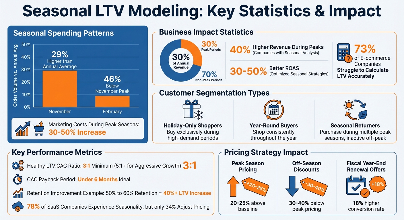
- Seasonal Spending Patterns: November sees 29% higher orders than the annual average, while February dips 46% below the November peak.
- Marketing Costs: Ad expenses can rise 30-50% during peak seasons, but smarter allocation can boost returns.
- Customer Segmentation: Distinguish between holiday-only shoppers, year-round buyers, and seasonal returners to tailor marketing efforts.
By combining historical data, cohort analysis, and advanced tools like BG/NBD models, businesses can predict customer behavior more accurately, optimize budgets, and even refine pricing strategies for peak and off-peak periods. Seasonal LTV insights help you focus on high-value customers, improve forecasts, and avoid misclassifying temporary inactivity as churn.
The takeaway? Seasonal LTV modeling isn’t just about tracking trends – it’s about using them to make smarter decisions year-round.
Seasonal LTV Modeling: Key Statistics and Customer Segments for E-commerce Success
Understanding Spend, aMER, & Spending Power
sbb-itb-2ec70df
Finding and Analyzing Seasonal Patterns
To build a seasonal LTV model, the first step is identifying when and where seasonality appears in your customer data. This requires digging deeper than just total revenue and spotting recurring yearly patterns. Luckily, you don’t need advanced statistical skills – just a solid approach and enough historical data to pinpoint genuine cycles.
How to Detect Seasonal Trends in Customer Data
Start by visually analyzing your data. Plot metrics like revenue, order volume, or acquisition rates over time to identify repeating patterns. A seasonal subseries plot, for example, compares the same months across different years. If January 2024 and January 2025 both show a similar dip, you’re likely seeing true seasonality rather than random variation.
For a more quantitative approach, use the Autocorrelation Function (ACF) to measure how data points are related at different time lags. If you’re working with monthly data, a spike at lag 12 signals annual seasonality. Decomposition methods can further break your data into its key components: the trend, seasonal pattern, and random noise. Use additive decomposition when seasonal changes are steady, or multiplicative decomposition if seasonal swings grow with your business size.
Cohort analysis is especially useful for e-commerce. Group customers by their first purchase date – like those acquired during Black Friday – and track their repeat purchase rates over 30, 60, and 90 days. Compare these cohorts with those acquired during slower months, such as February. This can reveal whether holiday shoppers are bargain hunters or if they stick around as loyal customers. Pairing this with RFM segmentation (Recency, Frequency, Monetary value) provides even more insight into customer behavior.
These techniques pave the way for using specific tools and statistical methods, which we’ll explore in the next section.
Tools and Methods for Seasonal Analysis
You don’t need pricey software to uncover seasonal trends. Python’s Statsmodels library offers tools like seasonal_decompose() and STL() for breaking down time-series data, while R users can rely on stl() and decompose(). Even Excel can handle basic seasonal forecasts using formulas like: Seasonal Forecast = Base Demand × Seasonal Index.
For more advanced analysis, SARIMA (Seasonal Autoregressive Integrated Moving Average) models account for both short-term changes and recurring seasonal cycles. If your data includes outliers or shifting trends, STL decomposition with Loess is more flexible. To validate your model, run a Ljung-Box test on the residuals. If seasonal patterns remain, your model may need further adjustment.
Marketing Mix Modeling (MMM) takes this a step further. It separates revenue driven by natural seasonal demand from revenue influenced by factors like advertising spend. Modern MMM platforms even update their models regularly, accounting for changes like inflation or shifts in consumer behavior.
Once you’ve clarified seasonal trends, the next step is to focus on grouping customers by their behavior.
Segmenting Customers by Seasonal Behavior
After identifying seasonal patterns, segment your customers into groups based on their purchasing habits. For instance:
- Holiday-Only Shoppers: Customers who buy exclusively during high-demand periods.
- Year-Round Buyers: Those who shop consistently throughout the year.
- Seasonal Returners: Customers who make purchases during multiple peak seasons but are inactive during off-peak times.
Tagging customers with their original acquisition source also helps track ROI over time. For example, if someone came through a Black Friday Facebook ad, maintaining that attribution lets you evaluate whether the acquisition cost was justified by their lifetime purchases.
For non-contractual e-commerce, consider using "Buy ‘Til You Die" (BTYD) models like BG/NBD. These models predict whether a customer is "alive" or "inactive" based on their recency and purchase frequency. Unlike linear retention models, BTYD is better suited for customers who might go inactive for months before returning during a peak season. Use SQL to extract key metrics such as recency (time since last purchase), frequency (number of purchases), T (total observation period), and average transaction size.
Segmenting customers by their seasonal behavior sets the stage for developing more tailored LTV models in later steps.
Building Seasonal LTV Models
Once you’ve identified seasonal patterns and divided your customers into segments, it’s time to create models that capture how these patterns influence customer value. Traditional LTV calculations often fall short here. The basic formula – LTV = Average Order Value × Purchase Frequency × Customer Lifespan – assumes customers purchase at a steady rate, which isn’t realistic for businesses with seasonal trends.
To address this, shift from linear retention models to probabilistic ones. These models recognize that customers may not have permanently churned after a period of inactivity; they could simply be between buying cycles. As Twilio Segment puts it:
"The retention rate is a linear model that doesn’t accurately predict whether a customer has ended her relationship with the company or is merely in the midst of a long hiatus between transactions".
Incorporating metrics like Recency and T (time since the last purchase) helps differentiate between seasonal breaks and actual churn.
Adjusting Basic LTV Formulas for Seasonality
To make standard LTV formulas work for seasonal businesses, move beyond simple averages. Start by calculating LTV over shorter, specific timeframes – such as weekly transaction rates – to better capture fluctuations throughout the year. For example, projecting over 26 weeks or 12 months can reveal how purchase frequency changes seasonally.
Another crucial step is applying a discount rate to future purchases. A common approach is using a 12.7% annual discount rate (or 1% monthly) to adjust future seasonal transactions to their present value.
Treating customers as individuals rather than averages significantly improves LTV accuracy. In one study, probabilistic modeling calculated a median LTV of $21.32, nearly double the simple average of $11.67. This highlights how advanced models can better account for the value generated by top-tier customers.
Advanced Predictive Models for Seasonal Data
For handling seasonality, Buy ‘Til You Die (BTYD) models outperform linear methods. A popular choice is the BG/NBD model (Beta-Geometric/Negative Binomial Distribution), which predicts future transactions based on frequency, recency, and tenure. Pair this with the Gamma-Gamma model to estimate the monetary value of those transactions. These models can predict outcomes ranging from 0.128 to over 16 transactions in 26 weeks, reflecting the diversity in customer behavior.
Before applying the Gamma-Gamma model, check the Pearson correlation between purchase frequency and monetary value. If frequent buyers also spend more, adjustments may be needed to ensure accurate results.
For implementation, Python’s lifetimes library offers tools like BetaGeoFitter for transaction predictions and GammaGammaFitter for transaction values. Combine these using the customer_lifetime_value() function. When working with smaller datasets, use a penalizer_coef (typically between 0.001 and 0.1) to avoid overly large parameter estimates.
To keep your models accurate, track metrics like MAE (Mean Absolute Error) and RMSE (Root Mean Square Error). If these exceed acceptable thresholds, it may indicate seasonal shifts or behavioral changes, signaling the need to retrain your model. For e-commerce brands, updating models monthly or quarterly is especially important during peak holiday seasons.
These predictive tools allow you to build features that capture the nuances of seasonal customer behavior.
Creating Features for Seasonal Models
The features you include in your model are crucial for capturing seasonal trends. Beyond standard RFM metrics (Recency, Frequency, Monetary value), consider adding binary flags for major shopping events like Black Friday, Cyber Monday, or back-to-school sales. These markers help identify natural demand spikes.
Incorporate product-specific seasonality features, such as Halloween costumes or Valentine’s Day flowers, to distinguish temporary peaks from ongoing trends. Additionally, segment features by customer demographics and location to uncover shared preferences that shift with the seasons.
For more advanced models, include macroeconomic factors like inflation rates, unemployment levels, or cost-of-living data. These variables provide context for shifts in purchasing power and behavior beyond the calendar. When analyzing marketing activities, separate branded and generic paid search efforts, as they serve different purposes during peak seasons.
To refine your model further, use dynamic ROI coefficients. These allow marketing effectiveness to vary daily or seasonally, rather than assuming a static return. For instance, Gaussian Process priors can link today’s ROI to both recent performance and historical data from the same date last year. As Tom Vladeck from Recast explains:
"Your marketing performs better when demand is high".
This method helps distinguish between base demand (sales that would happen anyway) and marketing-driven sales, ensuring seasonal effects aren’t over-credited while marketing efforts aren’t underappreciated.
Before training your model, remove outliers caused by unusual events, such as natural disasters or pandemics, which can distort seasonal patterns. For reliable seasonality analysis, aim to use at least two years of daily or weekly historical data.
Using Seasonal LTV Insights to Grow Your Business
Seasonal LTV models shine when they inform marketing investments, pinpoint the best times for promotions, and fine-tune pricing strategies. By understanding how customer value changes throughout the year, you can make smarter decisions about where to allocate your marketing budget, when to launch campaigns, and how to structure your pricing.
Segmenting Customers by Seasonal LTV
This approach goes beyond simply observing seasonal behavior. Instead, it uses predictive LTV to guide marketing investments. Customers don’t all behave the same way – some shop exclusively during Black Friday, while others maintain steady spending habits year-round. Grouping customers based on their seasonal behavior allows you to craft campaigns tailored to their buying patterns.
To predict future value, use BTYD models to rank customers by their likelihood of making future purchases. Then, divide them into PLTV deciles: deciles 01-02 as high, 03-09 as medium, and 10-20 as low future value.
- High-value customers: Use premium channels like Facebook ads or direct mail to maximize ROI. Treat these customers like VIPs, offering perks such as personal outreach or exclusive events.
- Medium-value customers: Focus on standard nurturing tactics and targeted promotions.
- Low-value customers: Minimize spending on costlier channels to avoid wasting resources on customers unlikely to convert.
Beyond value tiers, look at behavioral patterns. For example, identify "Early Bird" shoppers who buy before the holiday rush or those who only respond to discounts. Dive into the habits of your top 10% LTV customers – analyzing their order frequency or average purchase size can help you automate similar campaigns for prospective customers.
These refined segments not only guide where to spend your budget but also improve your ability to forecast revenue.
Allocating Budgets and Forecasting Revenue
Seasonal LTV predictions take the guesswork out of budget planning. Businesses that excel in analyzing seasonal trends often see 40% higher revenue during peak periods compared to those relying on intuition. The secret lies in knowing when to ramp up spending and when to hold back.
For e-commerce businesses, peak shopping periods can account for up to 30% of annual revenue, but they also come with challenges like a 20-50% increase in ad costs due to heightened competition. Shifting budgets to owned media channels during these high-demand periods can help drive organic conversions and reduce costs. Companies that fine-tune their seasonal strategies often achieve 30-50% better ROAS during these times.
Michelle Williams, Product Marketing Lead at Flieber, highlights the importance of this approach:
"Seasonality forecasting is not about predicting demand spikes. It’s about deciding when to accelerate demand and when pulling back is the smarter move".
To allocate budgets effectively, use NPV calculations on predictive LTV segments. Forecast future transactions, multiply by the average order size, and apply a 10% discount rate to rank customers. This helps you focus your resources where they’ll have the most impact.
Build multiple seasonal forecasts based on different market scenarios, giving you the flexibility to adapt if conditions change unexpectedly. Start this process early – well ahead of peak seasons – so you have time to plan, secure financing, or adjust inventory levels.
Adjusting Pricing and Promotions for Seasons
Seasonal LTV insights aren’t just for budget planning – they’re also key to pricing strategies. When customer demand varies throughout the year, static pricing can leave money on the table. Aligning your pricing with demand cycles can boost revenue during peak periods and help manage inventory during slower months.
- Peak seasons: Use premium pricing, increasing rates by 20-25% above baseline to capitalize on heightened demand. Instead of offering discounts, focus on "Value-Adjusted Packaging" by adding features or support to justify higher prices. For SaaS businesses, consider "Burst Capacity" pricing, which allows temporary usage increases during busy periods without requiring a permanent upgrade.
- Slow seasons: Offer significant discounts – 30-40% below peak pricing – to maintain sales momentum and clear inventory. For B2B businesses, align contract renewals with fiscal year-end budgets, as renewal offers made 2-3 months before the fiscal year ends have an 18% higher conversion rate than those made mid-year.
Develop a seasonal pricing calendar that outlines product-specific price changes and ensures smooth transitions between pricing tiers. Gradual adjustments prevent customer pushback and maximize revenue during these periods.
Despite the advantages, 78% of SaaS companies experience seasonality, yet only 34% actively adjust their pricing strategies to reflect these patterns. As Monetizely emphasizes:
"The most successful implementations treat seasonal pricing not as occasional discounting but as a fundamental strategic approach to value delivery".
Use elasticity analysis to determine how customers respond to price changes during different seasons. In peak periods with low price sensitivity, you can increase prices without significantly affecting sales volume. AI-powered tools can also help you test and refine pricing in real-time based on seasonal trends.
Measuring and Improving Seasonal LTV Models
Creating a seasonal LTV model is just the beginning. The real challenge lies in keeping it accurate as customer behavior and market conditions shift over time. Regular tracking and adjustments are crucial to ensure your model stays relevant and reliable.
Key Metrics for Evaluating Seasonal LTV Models
To evaluate your seasonal LTV model, focus on metrics that directly affect profitability. One critical measure is the LTV:CAC ratio. For a healthy e-commerce business, this ratio should be at least 3:1. If it reaches 5:1 or higher, there’s potential for aggressive growth strategies. Another key metric is the CAC payback period – if it exceeds six months, it may signal inefficient spending.
"LTV defines your acquisition ceiling. If your average customer is worth $120 in lifetime profit, you can’t sustainably spend $100 to acquire them." – Rework 2026 Guide
To gauge model accuracy, statistical tools like Mean Absolute Error (MAE), Root Mean Squared Error (RMSE), and R-squared are invaluable. These metrics show how closely your predictions align with actual customer behavior. Scatter plots comparing predicted and actual LTV values can also reveal accuracy – clusters near a diagonal line indicate strong performance.
Retention is another critical factor. For example, improving retention from 50% to 60% can increase LTV by over 40%. A jump from 70% to 80% results in a 51% boost. However, keep an eye on data drift (changing seasonal buying patterns) and concept drift (shifts in how variables like purchase frequency contribute to value). These changes can disrupt your model’s accuracy, and they’re a common challenge – 73% of e-commerce companies struggle to calculate Customer Lifetime Value due to such shifts.
Using cohort analysis – grouping customers by their acquisition month – can provide deeper insights into seasonal behaviors.
Historical vs. Predictive Seasonal LTV Models
The type of model you choose – historical or predictive – can significantly influence your ability to act on seasonal insights. Historical models rely on past transactions and realized profits, making them ideal for post-mortem analysis. Predictive models, on the other hand, estimate future customer behavior using techniques like machine learning (ML) or Recency, Frequency, and Monetary (RFM) signals, enabling real-time decision-making.
| Feature | Historical LTV Models | Predictive LTV Models |
|---|---|---|
| Data Basis | Actual past transactions and realized profit | Estimated future purchases using ML or RFM signals |
| Key Strength | Validates assumptions with high accuracy | Enables real-time decisions for budgeting and scaling |
| Limitations | Requires extensive historical data (12–24 months) | Can be skewed by overly optimistic inputs |
| Data Requirements | Long-term cohort data | Immediate calculation for new cohorts |
| Best Use Case | Benchmarking actual performance | Scaling marketing spend and acquisition strategies |
For e-commerce, predictive models using "Buy ‘Til You Die" (BTYD) logic are often more effective. These models assess whether a customer is "alive" or "dead" based on transaction patterns, avoiding the assumption of a linear retention rate. Historical models, by contrast, may misinterpret temporary inactivity as permanent churn.
Refining Your Seasonal LTV Models Over Time
To keep your seasonal LTV model aligned with changing trends, consistent evaluation and refinement are essential. Start by comparing predictive LTV scores from six months ago with actual revenue data to check the model’s accuracy. Regularly retrain your model – monthly or quarterly – with updated data to account for evolving seasonal patterns.
"Failing to capture changing trends [data drift] degrades the model’s accuracy and provides inaccurate predictions." – Deval Shah, Coralogix
Refinement should go beyond transaction history. Include additional features like web behavior (session duration, abandoned carts) and email engagement metrics (open and click rates). Early indicators, such as a high first-order AOV or a second purchase within 30 days, can help identify high-LTV customers early.
After seasonal adjustments, test your model’s residuals using the Ljung-Box test to ensure any remaining irregularities are random. Seasonal adjustment methods can reduce forecast errors by 10–15%, and even a modest 10% improvement in accuracy can lower inventory costs. To avoid misinterpreting one-off events as trends, handle outliers with robust decomposition techniques.
Conclusion
Seasonal LTV modeling isn’t just a buzzword – it’s a game-changer for marketing, inventory planning, and customer retention. By understanding how customer value shifts throughout the year, businesses can make smarter decisions: allocating budgets where they’ll have the most impact, keeping shelves stocked without overcommitting, and identifying which customers deserve extra attention. The difference between businesses that thrive and those that falter often boils down to planning ahead for seasonal trends rather than scrambling to react.
Yet, 73% of e-commerce companies struggle to calculate Customer Lifetime Value accurately. Why? Many overlook how seasonality influences customer behavior. Traditional models assume a static impact of marketing throughout the year, missing the chance to dynamically adjust for peak seasons. With seasonal LTV modeling, you can credit your marketing efforts appropriately during high-traffic periods and allocate resources when they matter most.
The real strength of seasonal LTV modeling lies in its ability to differentiate between customer types. For example, BTYD models help distinguish between customers who take seasonal breaks and those who are truly gone for good. This means you won’t mistakenly write off holiday shoppers who are likely to return next year, and you can focus retention efforts on customers who show signs of actual churn. Early indicators like a high first-order value or a quick follow-up purchase can even help you spot future VIPs before they’ve fully proven their worth.
Consumer habits change, markets evolve, and economic conditions shift. For seasonal businesses, keeping inventory at about 70% of peak-season levels can strike the right balance – avoiding stockouts while keeping costs under control. The companies that succeed aren’t the ones with perfect models from day one; they’re the ones that treat modeling as a continuous process of learning and fine-tuning.
Seasonal LTV modeling ties together the strategies discussed in this guide. It turns guesswork into strategy, helps balance revenue across busy and slow times, and ensures you’re investing in the right customers at the right moments. At Growth-onomics, we’re dedicated to helping businesses harness these insights to make smarter decisions and achieve sustainable growth.
FAQs
How does seasonal LTV modeling enhance marketing strategies?
Seasonal Lifetime Value (LTV) modeling gives you a clearer picture of how customer spending patterns shift throughout the year. By tapping into these seasonal trends, you can better plan your campaigns, allocate your marketing budget where it counts, and craft messages that resonate during peak spending periods.
This method also helps you separate long-term patterns from short-term seasonal changes, ensuring your decisions are backed by reliable data. When you add predictive analytics to the mix, you gain the ability to make real-time adjustments, refine customer segments, and allocate resources more effectively. The result? A stronger ROI and better customer retention. With these insights, businesses can make smarter decisions that drive consistent growth.
What are the best ways to identify seasonal trends in customer data?
To identify seasonal trends in customer data, you can rely on time series analysis techniques such as seasonal decomposition, autocorrelation, and seasonal subseries plots. These approaches make it easier to spot patterns that occur regularly over specific timeframes, like months or quarters.
Tools like Python’s statsmodels library or R’s forecasting packages are particularly useful for breaking data into seasonal components and recognizing recurring trends. You can also incorporate seasonality into your models by using dummy variables or accounting for calendar effects, which helps quantify how these patterns influence customer behavior. By doing so, you can improve demand forecasts and fine-tune lifetime value models to reflect seasonal shifts more accurately.
How can I adapt my Lifetime Value (LTV) models to account for seasonal customer behavior?
To fine-tune your LTV models for seasonal customer behavior, it’s important to weave seasonality directly into your analysis. Start by spotting patterns in your data – like spikes in activity during holidays or other peak periods – and adjust your models to mirror these trends. Using techniques such as decomposition methods (either additive or multiplicative) or advanced tools that isolate seasonal effects can sharpen your forecasts.
Recognizing multiple seasonal trends, such as the rush before holidays or slower periods afterward, adds another layer of accuracy to your models. By factoring in these fluctuations, your LTV predictions will stay reliable throughout the year, helping you craft smarter marketing strategies, allocate resources more effectively, and make better decisions overall. This approach also separates genuine performance changes from temporary seasonal shifts, offering a more accurate view of your customers’ behavior.