

Price elasticity of demand (PED) measures how much demand changes when prices shift. It’s calculated by dividing the percentage change in quantity demanded by the percentage change in price. This metric helps businesses decide if price changes will increase or decrease revenue. Here’s a quick breakdown of five methods to calculate PED:
- Basic Percentage Change Formula: A simple way to estimate elasticity using initial and new price/quantity values. Best for small price changes but less reliable for large shifts.
- Midpoint Method: Solves directional bias by averaging price and quantity values. Useful for consistent results across price ranges.
- Point Elasticity: Uses calculus to find elasticity at a specific price point. Ideal for precise adjustments but requires a defined demand function.
- Regression Analysis: Incorporates multiple variables like seasonality and competitor pricing for detailed insights. Requires extensive historical data and statistical tools.
- Experimental/Survey Methods: Tests consumer reactions through price experiments or surveys, especially helpful for new products or markets.
Each method fits different pricing scenarios, from quick estimates to complex analyses. Choosing the right one depends on your data availability, tools, and goals.
Price Elasticity of Demand: 5 Calculation Methods Comparison
Calculating the Elasticity of Demand
1. Basic Percentage Change Formula
The Basic Percentage Change Formula is a straightforward way to calculate price elasticity of demand. It works by dividing the percentage change in quantity demanded by the percentage change in price, using the initial values. The formula looks like this:
(Q₂ – Q₁) / Q₁
(P₂ – P₁) / P₁
To use it, you’ll need four numbers: the initial price (P₁), the new price (P₂), the initial quantity demanded (Q₁), and the new quantity demanded (Q₂). For instance, imagine you sold 100 units at $10.00, but after raising the price to $12.00, sales dropped to 80 units. Plugging these values into the formula gives you the elasticity. This method serves as a foundation for more advanced techniques discussed later.
Data Requirements
You only need two price points and their corresponding sales figures. No fancy software, statistical tools, or large datasets are necessary.
Best Use Case
"For rough approximations use the point method; for greater accuracy, the midpoint method." – Lumen Learning
This formula works well for quick, rough estimates, especially when analyzing small price changes. It’s most effective when the two data points are close together on the demand curve, providing a general idea of how customers might react to slight price adjustments.
Technical Complexity
The calculations are simple and require just basic arithmetic – no specialized tools or expertise are needed. This makes it a handy option for gaining quick insights without the need for a data analyst.
Common Pitfalls
One common issue is directional inconsistency. Measuring a price change in one direction can yield a different result than measuring it in reverse. This "index number problem" can lead to varying elasticity results depending on the direction of the change.
Another limitation is accuracy. The formula becomes less reliable when dealing with significant price changes. It’s better suited for small adjustments, as larger shifts can distort the results.
2. Midpoint Method Arc Elasticity
The midpoint method, often called arc elasticity, solves the issue of directional inconsistency found in the basic percentage change formula. Instead of relying on initial values, this method uses averages, ensuring consistent elasticity results no matter the direction of the price change.
To calculate elasticity, divide the percentage change in quantity (based on the average of Q₁ and Q₂) by the percentage change in price (based on the average of P₁ and P₂). For instance, imagine T-shirt prices rising from $14.00 to $16.00 (average $15.00) while sales drop from 60 to 40 units (average 50). Using this method, the elasticity comes out to 3.0, reflecting highly elastic demand.
"The advantage of the midpoint method is that one obtains the same elasticity between two price points whether there is a price increase or decrease." – Lumen Learning
Data Requirements
To use this method, you’ll need four data points: P₁, P₂, Q₁, and Q₂.
Best Use Case
This approach works well for estimating elasticity across a price range. It delivers consistent results regardless of whether prices rise or fall, though it assumes the demand curve is roughly linear between the two data points.
Technical Complexity
Although the midpoint method adds the step of calculating averages, it only requires basic arithmetic.
Common Pitfalls
One common mistake is confusing elasticity with the slope of the demand curve. While the slope of a linear demand curve remains constant, elasticity changes at different points along the curve. Another limitation is that the midpoint method can only handle two data points at a time. For multiple price changes, you’ll need to calculate elasticity separately for each pair. Up next, we’ll dive into point elasticity, which uses calculus to calculate elasticity at a specific point on the demand curve.
3. Point Elasticity from a Demand Function
Point elasticity uses calculus to measure how demand responds to price changes at a specific price point. Unlike other methods, it focuses on elasticity at a single price by calculating the slope of the demand function. The formula for point elasticity is:
Eₚ = (dQ/dP) × (P/Q)
This approach helps identify the price that maximizes revenue – where demand becomes unit elastic (elasticity equals -1). At this point, the impact of price changes is perfectly balanced by changes in quantity demanded.
"The point elasticity can be computed only if the formula for the demand function, $Q_d = f(P)$, is known so its derivative with respect to price, $dQ_d/dP$, can be determined." – Wikipedia
Data Requirements
To calculate point elasticity, you need three key pieces of information:
- A defined demand function (e.g., Q = f(P))
- The specific price and quantity at the point of interest
- The ability to compute the derivative of the demand function
In many cases, the demand function is built using regression analysis or advanced statistical techniques.
Best Use Case
Point elasticity is ideal for continuous models where small price changes significantly influence demand. It’s particularly effective in industries like luxury goods or electronics, where minor price adjustments near certain thresholds can lead to noticeable shifts in consumer behavior.
Technical Complexity
This method involves differential calculus, making it more technically challenging than simpler percentage-based methods. Building a reliable demand model is critical, as even small errors in calculating the derivative can lead to inaccurate results.
Common Pitfalls
Be cautious about assuming elasticity remains constant along the demand curve. Even linear demand curves can show varying elasticity at different price points. Additionally, external factors like marketing efforts or competitor pricing can skew results, making it essential to account for these influences.
Up next, we’ll dive into regression-based methods that incorporate multiple variables to provide more nuanced elasticity estimates.
sbb-itb-2ec70df
4. Regression-Based Elasticity Estimation
Unlike simpler methods that focus solely on direct price-quantity changes, regression analysis takes a broader perspective. It uses econometric models to untangle the impact of price from other demand factors, such as promotions, seasonality, advertising, and competitor pricing. By incorporating these variables, regression-based elasticity offers a more detailed understanding of what drives demand, helping businesses make smarter pricing decisions.
One example comes from October 2008, when Chamberlain Economics analyzed retail gasoline data from 2000–2007 using regression methods. By factoring in seasonal variations, they estimated a short-run price elasticity of -0.048.
Data Requirements
For regression analysis to work effectively, you need historical sales data paired with corresponding price levels. To separate the effect of price changes, you’ll also need to include control variables like:
- Promotions
- Advertising efforts
- Seasonal trends
- Competitor pricing
- Macroeconomic indicators (e.g., disposable income, inflation)
Data can be structured as time series, cross-sectional, or panel data. Among these, panel data often delivers the most reliable insights because it captures both time-based and cross-sectional variations.
Best Use Case
Regression models shine in environments rich with data, especially when detailed Point of Sale (POS) information is available. They’re particularly useful during competitive periods, like price wars, where understanding the interplay of multiple factors – including cross-price effects – is critical. Since these models can be updated regularly (monthly or quarterly), they’re ideal for ongoing price optimization rather than one-off analyses.
Technical Complexity
This approach demands careful attention to technical details. For instance, choosing the right functional form is crucial – double-log models are a common choice because their coefficients directly represent elasticities. Another challenge is addressing endogeneity, where price and sales influence each other. Techniques like instrumental variables are often used to resolve this. Depending on the data type, different estimators might be required, such as Logit or Probit models for discrete choices or autoregressive models for time series data.
Common Pitfalls
Several challenges can undermine the accuracy of regression-based elasticity estimates. For example:
- Limited price variation in historical data: Without enough variation, it’s tough to pinpoint the true effect of price changes.
- Omitted variable bias: Ignoring factors like competitor actions or economic trends can skew results.
- Outdated models: Elasticity isn’t static – it evolves with technology, consumer behavior, and market conditions. Relying on old models for long-term forecasting can lead to errors.
To avoid these issues, regular model updates and the inclusion of relevant control variables are essential.
5. Experimental and Survey-Based Elasticity
When historical data isn’t available or you’re testing pricing strategies before rolling them out widely, experimental and survey methods can provide direct insights into consumer responses. These approaches involve controlled price changes or asking customers directly about their preferences. While they can yield useful results, they do require careful planning to avoid potential pitfalls.
Take Netflix‘s 2011 price experiment, for example. The company raised the cost of its streaming and DVD rental package by about 60%, jumping from $10.00 to $15.98 per month. This move served as a natural experiment, revealing how many customers would leave versus how many were willing to pay the higher price. Governments also use similar strategies, like applying "sin taxes" on cigarettes. In the U.S., cigarette taxes vary widely – from 17 cents per pack in Missouri to $4.35 per pack in New York – offering opportunities to study consumer behavior across state lines.
Data Requirements
To make these methods work, you’ll need to gather specific data. This includes the initial and adjusted price points, the corresponding quantities sold, and additional details like the availability of substitutes, the share of the product in household budgets, and the timeframe for consumer responses. For surveys, you’ll need to present customers with different product bundles at varying price levels and record their likelihood of making a purchase.
It’s also important to note that elasticity often differs over time. For instance, U.S. crude oil showed a short-run elasticity of -0.061, while its long-run elasticity climbed to -0.453. These distinctions highlight the importance of detailed data collection to ensure accurate and meaningful results.
Best Use Case
Experimental and survey-based methods are particularly effective when introducing new products, entering unfamiliar markets, or testing pricing strategies in a controlled environment. They’re also invaluable for exploring psychological factors that go beyond straightforward price sensitivity. Tools like conjoint analysis, which asks consumers to evaluate product bundles at different price points, can simulate real-world trade-offs more effectively than simply asking about price preferences.
Technical Complexity
Though the concept behind these methods is relatively simple, executing them properly often requires advanced tools like conjoint analysis software and visualization platforms to interpret consumer behavior accurately. One major challenge is the "say-do" gap – what people claim they’ll do doesn’t always match their actual behavior. Gill Avery, a Senior Lecturer at Harvard Business School, explains:
"The challenge is that what people say they will do is not what they actually do when they are standing at the shelf".
Such insights are crucial for refining these methods and complementing other elasticity measurement techniques.
Common Pitfalls
Experimental and survey methods can be time-intensive and resource-heavy compared to mathematical approaches. They may also miss complex market factors, like competitors’ reactions or sudden shifts in consumer sentiment. To counter these challenges, segmenting data by demographics or behavior and using AI-powered analytics can help track real-time influences such as seasonality or marketing campaigns. These steps can improve the accuracy and reliability of your results.
Method Comparison Table
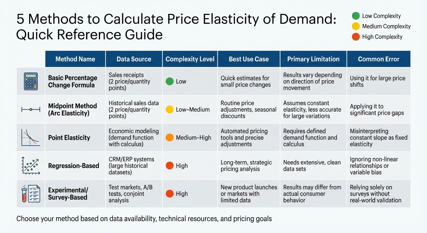
Selecting the right method to measure elasticity depends on the type of data you have, the technical tools at your disposal, and your pricing goals. Each method has its own advantages and challenges. Here’s a breakdown of five commonly used approaches, comparing them across key factors relevant to U.S. pricing strategies:
| Method | Data Source | Complexity Level | Best Pricing Application | Primary Limitation | Common Error |
|---|---|---|---|---|---|
| Basic Percentage Change | Sales receipts (2 price/quantity points) | Low | Quick estimates for small price changes | Results vary depending on the direction of price movement | Using it for large price shifts instead of the Midpoint Method |
| Midpoint (Arc Elasticity) | Historical sales data (2 price/quantity points) | Low–Medium | Routine price adjustments, such as seasonal discounts | Assumes constant elasticity, making it less accurate for large price variations | Applying it to significant price gaps |
| Point Elasticity | Economic modeling (demand function with calculus) | Medium–High | Automated pricing tools and precise adjustments | Requires a defined demand function and calculus | Misinterpreting the constant slope of a linear demand curve as fixed elasticity |
| Regression-Based | CRM/ERP systems (large historical datasets) | High | Long-term, strategic pricing analysis | Needs extensive, clean data sets | Ignoring non-linear relationships or variable bias |
| Experimental/Survey-Based | Test markets, A/B tests, conjoint analysis | High | Launching new products or entering markets with limited data | Results may differ from actual consumer behavior | Relying solely on survey responses without validating with real-world data |
Each method serves a specific purpose depending on the pricing scenario. For example, the Midpoint Method works well for tactical decisions, like adjusting prices during seasonal sales, as it offers reliable results without requiring advanced tools. On the other hand, experimental methods are indispensable when launching a new subscription service or entering a market where historical data is unavailable. For businesses with access to extensive datasets, regression analysis allows for isolating the effects of price changes while accounting for variables like competitor pricing, seasonality, and consumer income.
One important consideration is that elasticity is not static – it changes over time. This variability can significantly impact your planning, making it essential to align your elasticity measurement method with your planning horizon.
While the Basic Percentage Change Formula is handy for quick calculations, it’s less suitable for formal analysis due to its directional bias. It’s best reserved for rough estimates rather than detailed business decisions.
Conclusion
Price elasticity isn’t just a theoretical concept – it’s a practical tool that can directly shape your revenue outcomes. The five methods we’ve explored in this article cater to different business needs, from quick, straightforward calculations using the Basic Percentage Change Formula to detailed regression analysis for more strategic, long-term planning. The best approach depends on the data you have, the level of detail you need, and whether your pricing decisions are short-term adjustments or part of a bigger strategy.
Each method has its place. For instance, if you’re experimenting with a seasonal discount and only have limited data, the Midpoint Method provides dependable results without requiring advanced tools. On the other hand, launching a new product with little historical data might push you toward experimental or survey-based methods. If you’re managing a large inventory with thousands of SKUs, regression analysis can handle the complexity by accounting for variables like competitor pricing and seasonal trends – though it does demand a robust, clean dataset.
It’s also worth noting that elasticity isn’t static. It changes over time and varies by product. That’s why it’s crucial to revisit your calculations regularly instead of relying on one-time estimates. This ongoing evaluation helps turn pricing decisions from educated guesses into informed strategies.
At Growth-onomics, we specialize in crafting data-driven pricing strategies tailored to your market. Through advanced Data Analytics and Performance Marketing, we identify whether your products act as "profit generators" (inelastic, where price increases drive revenue) or "promotional powerhouses" (elastic, where discounts boost sales volume). This precision allows you to fine-tune pricing decisions across your entire product line, eliminating guesswork.
Ultimately, successful pricing strategies often involve a mix of methods. Whether you’re working with a small catalog or a sprawling inventory, understanding and applying the right elasticity calculations can turn pricing into a powerful competitive edge.
FAQs
What is the best way to calculate price elasticity of demand for my business?
The method you choose for calculating price elasticity of demand should align with your data, the size of the price change, and how precise your results need to be. If you only have two data points – like before and after a price discount – the simple percent-change formula is a quick option. However, keep in mind that results can vary depending on the base point you use. For most business needs, the midpoint (arc) method is a better choice since it provides consistent results, whether prices go up or down.
For deeper insights, you might consider point elasticity or regression-based elasticity. These methods are more advanced and require larger datasets or specialized tools. They’re especially useful for businesses with continuous demand curves or significant amounts of sales data.
To decide which method works best, start by evaluating your data. Use the midpoint method for basic price comparisons, or opt for regression-based approaches for more intricate pricing strategies. If you’re looking for expert guidance, Growth-onomics offers support in analyzing sales data and creating elasticity models to help you make smarter pricing decisions.
What mistakes should I avoid when using regression to estimate price elasticity of demand?
When estimating price elasticity using regression, there are several common challenges that can lead to inaccurate results if not addressed carefully.
First, keep in mind that price is often endogenous – it’s not just a driver of demand but also influenced by it. A simple regression that ignores this relationship can produce biased results. To tackle this, consider using approaches like instrumental variables or simultaneous-equations models to properly account for the interplay between price and sales volume.
Second, don’t forget about important control variables. Factors like promotions, seasonality, competitor pricing, and advertising can all affect sales. If these are left out of your model, you risk introducing omitted-variable bias, which can distort your understanding of how price changes truly impact demand.
Finally, pay close attention to data quality and model selection. Small or noisy datasets, using the wrong functional form (like a linear model when a log-log approach is more appropriate), or issues such as heteroskedasticity can undermine your results. Take the time to validate your data, check residuals, and test for problems like autocorrelation to ensure your estimates are as reliable as possible.
How does price elasticity change over time, and how can I use it to adjust pricing strategies?
Price elasticity isn’t a fixed concept – it shifts over time as factors like consumer income, market competition, seasonal patterns, and product availability change. Even on the same demand curve, elasticity can fluctuate at different price levels. For instance, the entry of a new competitor or a rise in disposable income can quickly alter how price-sensitive customers are.
To refine your pricing strategy, think of elasticity as a moving target. Regularly analyze it using up-to-date sales data and compare it with historical patterns. Break down your customer base by factors such as location, buying habits, or sales channel since elasticity often varies across different groups. If you notice demand becoming more elastic, offering discounts or bundling products can help sustain sales. On the other hand, when demand leans toward being inelastic, you might have room to increase prices or introduce premium offerings without significantly impacting sales. Using dynamic pricing tools and AI-driven forecasting can make it easier to track these shifts in real-time and experiment with pricing adjustments before rolling them out broadly.