
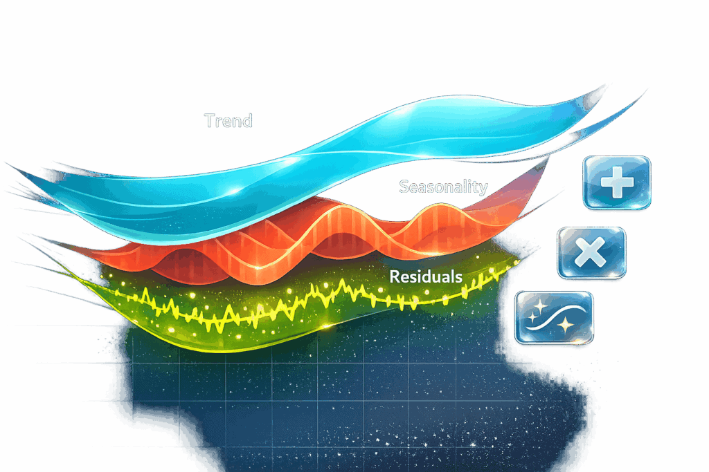
Decomposition methods are essential for understanding time series data by separating it into three components: trend, seasonality, and residuals. This helps businesses and analysts make sense of patterns, identify anomalies, and improve forecasting accuracy. Here’s what you need to know about the three main methods:
- Classical Additive Decomposition: Best for data with constant seasonal patterns. It separates components linearly but struggles with outliers and assumes fixed seasonality.
- Classical Multiplicative Decomposition: Suitable when seasonal variations grow or shrink with the trend, making it ideal for datasets like retail sales. However, it’s sensitive to anomalies and rigid in handling seasonality.
- STL Decomposition (Seasonal and Trend Decomposition Using Loess): Offers flexibility by allowing seasonal patterns to evolve over time. It’s robust against outliers but requires parameter tuning and works only with additive models unless transformed.
Each method has strengths and limitations, and the choice depends on your data’s characteristics. For instance, additive works well with steady seasonal patterns, while multiplicative handles proportional changes. STL is ideal for complex datasets with shifting trends and seasonality.
Quick Comparison
| Method | Best For | Limitations |
|---|---|---|
| Classical Additive | Stable seasonal patterns | Fixed seasonality; outlier sensitivity |
| Classical Multiplicative | Seasonal changes proportional to trend | Rigid seasonality; outlier sensitivity |
| STL Decomposition | Evolving trends and seasonality | Additive models only; requires tuning |
Understanding these methods can refine your forecasting approach and provide actionable insights for decision-making.

Comparison of Time Series Decomposition Methods: Additive, Multiplicative, and STL
Decomposition of Time Series into Trend, Seasonality & Residual from Scratch
sbb-itb-2ec70df
1. Classical Additive Decomposition
Classical Additive Decomposition is a method that has been around since the 1920s. It breaks down a time series into three distinct components:
yₜ = Sₜ + Tₜ + Rₜ
Here, Sₜ represents the seasonal component, Tₜ is the trend-cycle, and Rₜ accounts for the random fluctuations. By separating these elements, you can better understand patterns in your data – whether it’s monthly sales, website traffic, or another metric – and use that insight for forecasting.
"The classical decomposition method originated in the 1920s. It is a relatively simple procedure, and forms the starting point for most other methods of time series decomposition." – Rob J Hyndman and George Athanasopoulos, Authors of Forecasting: Principles and Practice
Trend Estimation
The trend component is calculated using moving averages. For data with an even seasonal period – like monthly data with a 12-month cycle – a 2×12 moving average is applied to center the trend around each observation. For an odd seasonal period (e.g., weekly data with a 7-day cycle), a simple m-period moving average is used. Once the trend is estimated, subtracting it from the original series leaves you with the non-trend components.
Handling Seasonality
To account for seasonality, the detrended data is grouped by period (e.g., all January values, all February values, etc.), and the averages for each period are computed. These averages are then adjusted to sum to zero, ensuring the seasonal effects are balanced over the cycle. One limitation of this method is its assumption that seasonal patterns remain unchanged over time.
"The additive decomposition is the most appropriate if the magnitude of the seasonal fluctuations, or the variation around the trend-cycle, does not vary with the level of the time series." – Rob J Hyndman and George Athanasopoulos, Authors of Forecasting: Principles and Practice
Computational Simplicity
This method relies on basic calculations – moving averages, subtractions, and simple averaging – making it efficient and easy to implement. However, it does come with a few challenges. For instance, trend estimates are not available for the start and end of the series. Using monthly data as an example, the first and last six observations lack trend estimates. Additionally, the method is sensitive to outliers, meaning an unexpected event can skew the seasonal averages.
Despite its limitations, the Classical Additive Decomposition method remains a foundational tool for understanding time series data. It sets the stage for exploring more advanced decomposition techniques, such as the Classical Multiplicative Decomposition method.
2. Classical Multiplicative Decomposition
Classical Multiplicative Decomposition is built on the idea that seasonal variations grow in proportion to the trend: yₜ = Tₜ × Sₜ × Rₜ. This makes it especially useful for datasets where seasonal fluctuations increase alongside the overall trend. For instance, retail sales during the holiday season often grow not just in absolute terms but also as a percentage of total annual revenue. Unlike the additive model, this approach adjusts for proportional seasonal changes, making it a better fit for such scenarios.
"Multiplicative decomposition is used when the magnitude of seasonal and irregular variations is related to the trend level." – Pankaj Das and Samir Barman
Trend Estimation
Estimating the trend in the multiplicative model involves a similar process to the additive approach but with a key difference: instead of subtracting the trend, you divide it to maintain proportionality. Moving averages are still the go-to method for trend estimation. For even periods, use a 2×m moving average; for odd periods, use an m-period average. Once the trend is calculated, divide the observed values (yₜ) by the trend to separate out the seasonal and random components.
Handling Seasonality
To address seasonality, divide the series by its trend values and then calculate the average of these detrended values for each period. Adjust the resulting seasonal indices so they sum to the number of periods (m). A practical example of this method comes from 2016, when researchers in Iran applied it to forecast biohydrogen production from agricultural crop residues. They fine-tuned the moving average length by comparing forecasts to actual historical data.
Flexibility
While the multiplicative model provides a useful framework, it shares some of the limitations of its additive counterpart. It assumes that seasonal patterns repeat consistently over time and can be highly sensitive to outliers. A single unexpected event could skew the seasonal indices, leading to distorted results.
Computational Complexity
This method remains straightforward, relying on basic calculations like moving averages, division, and averaging. However, as with the additive model, it struggles with edge cases where trend estimates are unavailable and may oversmooth rapid changes in the data.
3. STL Decomposition (Seasonal and Trend Decomposition Using Loess)
STL relies on Loess smoothing to break down time series data, capturing non-linear trends and evolving seasonal patterns. Introduced in 1990, it adapts well to a variety of data behaviors, making it more versatile than classical methods.
"STL is a versatile and robust method for decomposing time series… the smoothness of the trend-cycle can also be controlled by the user." – Rob J Hyndman, Professor of Statistics, Monash University
Trend Estimation
STL estimates trends using Loess smoothing instead of simple moving averages. The trend window parameter gives you control over how responsive or stable the trend appears. A smaller trend window tracks rapid changes, while a larger one results in smoother trends. For monthly data, the default trend window is typically set at 21. Adjustments to this parameter can help fine-tune how well the trend captures the underlying signal.
Handling Seasonality
Unlike older methods that assume seasonal patterns are fixed, STL allows the seasonal component to change over time. You can adjust the rate of this change using the seasonal window parameter. This flexibility enables STL to handle various seasonal cycles, whether hourly, daily, weekly, or custom-defined. In contrast, traditional approaches like X-11 and SEATS are limited to monthly or quarterly data. A good rule of thumb for smoother results is to set the trend smoother length to about 150% of the seasonal smoother length.
Flexibility
STL provides significant customization through its user-defined parameters and includes a robust fitting option that minimizes the impact of outliers. This feature is especially useful when dealing with anomalies or unexpected events in your data. However, STL is designed for additive decompositions only. If your seasonal variation grows with the level of the series, you’ll need to apply a Box-Cox or log transformation before decomposition to handle multiplicative patterns effectively.
Computational Complexity
STL also tackles the computational challenges associated with non-linear smoothing. Loess smoothing, which involves local polynomial regressions, can be resource-intensive for large datasets. To improve efficiency, STL employs a "jump" mechanism, calculating Loess for every nth point and filling in the gaps with linear interpolation. Research shows that setting the jump parameter to 15% of the window length significantly speeds up processing with minimal impact on accuracy. The algorithm uses inner iterations (typically 2) to refine components and up to 15 outer iterations for robust fitting, particularly when managing outliers.
Pros and Cons
Every decomposition method has its own set of benefits and drawbacks. Classical additive decomposition stands out for its simplicity and ease of interpretation, making it a solid choice for grasping the basic components of time series data. That said, it struggles in practical scenarios because it assumes that seasonal patterns remain unchanged over time.
On the other hand, classical multiplicative decomposition is better equipped for economic datasets, where seasonal variations tend to scale with the underlying trend.
STL decomposition takes flexibility to the next level. It adapts to shifting seasonal patterns and handles outliers well, making it particularly useful for datasets with evolving trends. However, this method can be more demanding, requiring careful parameter adjustments and, in some cases, transformations like log or Box-Cox to address multiplicative relationships, as STL natively supports only additive models.
"While classical decomposition is still widely used, it is not recommended, as there are now several much better methods." – Rob J. Hyndman, Professor of Statistics
The choice of method boils down to the characteristics of your data. Additive models work best when seasonal fluctuations stay consistent, such as in some environmental datasets. In contrast, multiplicative models shine when seasonal variations grow or shrink in proportion to the trend, a common pattern in retail and economic data. For datasets with non-linear trends or spanning long time periods, STL provides superior results, albeit with more setup effort.
The table below provides a quick comparison of each method’s strengths, limitations, and ideal use cases:
| Method | Key Strengths | Key Weaknesses | Best Application |
|---|---|---|---|
| Classical Additive | Simple to calculate; clear linear separation | Struggles with missing data; assumes fixed seasonality; sensitive to outliers | Stable seasonal patterns over time |
| Classical Multiplicative | Effective for scaling seasonal changes | Issues with missing data; rigid seasonality; over-smooths rapid changes | Seasonal variation proportional to trend |
| STL Decomposition | Handles any seasonal period; adjusts to changes; robust to outliers; user-controlled smoothness | Requires parameter tuning; no automatic trading day handling; additive models only | Complex data with non-linear trends or evolving patterns |
Conclusion
Choose a decomposition method that aligns with your data’s characteristics. If seasonal patterns stay consistent over time, classical additive decomposition is the way to go. On the other hand, classical multiplicative decomposition is better suited for data like sales or economic trends, where seasonal peaks grow or shrink in proportion to the overall trend. For long-term datasets with shifting seasonal behaviors – like electricity demand, where peak usage changes seasonally – STL decomposition is a flexible option. It adjusts to evolving seasonality and handles outliers effectively, making it a strong choice for complex series. Your selection has a direct impact on the accuracy of forecasts and the reliability of your models.
Decomposing a time series before forecasting allows you to treat components separately. For example, the seasonal element can be modeled using a simple seasonal naïve method, while the seasonally adjusted data can be forecasted with tools like Holt’s method or ARIMA.
"STL has several advantages over classical decomposition… the seasonal component is allowed to change over time, and the rate of change can be controlled by the user." – Rob J. Hyndman and George Athanasopoulos
To determine the best approach, start by plotting your data. If seasonal variations grow as the trend increases, a multiplicative model or log transformation might work best. If the seasonal fluctuations remain steady, an additive model is more appropriate. Also, review the residuals for any autocorrelations – these could indicate that the decomposition didn’t fully capture the underlying patterns.
The right decomposition method transforms raw time series data into meaningful insights, setting the stage for more accurate forecasts and informed decision-making.
FAQs
How do I know if my seasonality is additive or multiplicative?
To figure out whether your seasonality is additive or multiplicative, look at how seasonal changes interact with the overall level of your time series.
- Additive seasonality means the seasonal variation stays consistent over time. It follows the formula:
Y(t) = T(t) + S(t) + E(t)
Here, seasonal effects are simply added to the trend and error components. - Multiplicative seasonality means the seasonal variation grows or shrinks in proportion to the series level. Its formula is:
Y(t) = T(t) × S(t) × E(t)
In this case, seasonal effects scale with the trend.
A quick visual check of your data can often reveal whether the seasonal patterns remain steady or change with the series level, helping you choose the right model for analysis.
What should I do about missing data before decomposing a time series?
Before breaking down a time series, it’s crucial to deal with missing data to keep results reliable. Outliers need careful attention – only replace them if they’re clear errors or highly unlikely to happen again. Missing values can be filled in or estimated in a way that fits the overall data pattern. Sometimes, transforming or adjusting the series beforehand can make the decomposition process smoother. Handling missing data and outliers thoughtfully leads to better-quality analysis.
How do I choose STL parameters like seasonal and trend windows?
When choosing STL parameters, keep these tips in mind:
- Seasonal window: Pick an odd number, with a minimum of 7. Larger numbers help smooth out seasonal patterns. If your data has fixed, repeating patterns, you can set this to "periodic".
- Trend window: This is usually 1.5 times the seasonal window and should also be an odd number. If you don’t specify it, defaults will be used.
- Low-pass window: Opt for the smallest odd number that’s higher than the frequency of your data. This helps minimize interference.
Test different combinations and visually review the results to find what works best for your data.