

Customer churn doesn’t happen instantly – it’s a gradual process that can often be predicted using time-series models. These models track changes in customer behavior over time, such as reduced logins, fewer purchases, or increased support tickets, to help businesses act before customers leave. Why does this matter? Retaining customers is far cheaper than acquiring new ones, and a slight increase in retention can significantly boost profits.
Here’s a quick breakdown of the process:
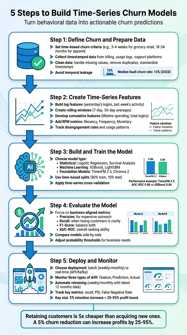
- Step 1: Define Churn and Prepare Data
Identify what churn means for your business and clean your time-series data to avoid errors or data leakage. - Step 2: Create Time-Series Features
Build features like lagged values, rolling averages, and RFM (Recency, Frequency, Monetary) metrics to capture behavioral trends. - Step 3: Build and Train the Model
Choose models like Logistic Regression, XGBoost, or advanced foundation models based on your goals. Use time-based splits to avoid bias. - Step 4: Evaluate the Model
Focus on metrics such as precision, recall, and AUC-ROC to ensure your model aligns with business objectives. - Step 5: Deploy and Monitor
Deploy predictions in real-time or batch processes and monitor for data drift to maintain accuracy.
5-Step Process for Building Time-Series Churn Prediction Models
Step 1: Define Churn and Prepare Your Data
Setting Time-Based Churn Criteria
Defining churn is the first critical step, especially when dealing with time-series data. Unlike subscription-based businesses where churn is clear (e.g., a canceled subscription), other industries must establish an "Attrition Trigger" – a specific period of inactivity that signals churn. For example, in grocery retail, churn might be triggered after 3–4 weeks of no activity. In contrast, an online athletic apparel retailer might define churn after 18–24 months of inactivity.
Instead of waiting for complete inactivity, focus on identifying declining engagement early. Waiting too long can make intervention impossible. As Guillaume Colley explains, "Predicting Dormancy is not an actionable insight". To set churn thresholds effectively, consider using the percentile method to calculate transaction intervals, ensuring minimal false positives. For seasonal businesses, a good rule of thumb is to double the typical seasonal cycle – for instance, using a 24-month trigger if purchases are usually annual. For customers with consistent purchasing patterns, personalized triggers based on a multiple of their average transaction interval can be helpful. As a reference point, the median churn rate for private SaaS businesses in 2022 was 13%.
Collecting and Cleaning Your Time-Series Data
Once churn is defined, the next step is to gather and clean your time-series data. Start by collecting timestamped data from sources like billing systems, product usage logs, and customer support platforms. At a minimum, your dataset should include a unique customer identifier and a transaction timestamp.
Be cautious of temporal leakage – this happens when data from after the churn event sneaks into your training dataset. It can artificially inflate model accuracy but won’t translate to real-world effectiveness. Clean your dataset by handling missing values, removing duplicates, and standardizing timestamps across time zones. To keep the data reliable, split it into "pre" and "post" observation windows, ensuring the training data remains uncontaminated.
Since churn events are usually rare (often affecting only about 10% of the dataset), you’ll also need to address class imbalance during the modeling process. By following these steps, you can create a dataset that accurately reflects customer behavior over time, setting a strong foundation for churn prediction.
sbb-itb-2ec70df
Time-Series Behavioral Analysis for Churn Prediction – Damon Danieli – ML4ALL 2019
Step 2: Create Time-Series Features
Once your data is clean, the next step is to build features that capture how and when customer behavior changes over time. Time-series modeling not only shows what customers do but also highlights the timing and frequency of their actions.
Building Lagged and Aggregated Features
Lag features are created by shifting variables by specific time intervals. For example, "Lag 1" might represent yesterday’s logins, while "Lag 7" could indicate activity from a week ago. These features help capture short-term patterns and recurring behaviors.
It’s important to fill any timeline gaps so that lag features always refer to the most recent time step, such as the previous day, rather than skipping over inactive periods. Rolling windows, like 7-day or 30-day averages, are another useful tool. They smooth out random fluctuations and highlight trends over shorter periods.
Cumulative features, on the other hand, track totals over the entire time series up to the current point. Examples include lifetime spending, cumulative logins, or averages that grow over time. These features help your model understand long-term patterns. When calculating these, stick to trailing or expanding methods to avoid data leakage.
| Feature Type | Purpose | Example |
|---|---|---|
| Lag Features | Captures short-term patterns and dependencies | Previous day’s activity or sales |
| Rolling Features | Highlights trends by smoothing out noise | 7-day moving average of engagement |
| Cumulative Features | Tracks long-term trajectories and totals | Total lifetime spend or logins to date |
These time-based features provide a strong foundation for analyzing customer behavior in greater depth.
Developing Behavioral and RFM Features
After creating lagged and aggregated features, you can refine your analysis by incorporating behavioral and RFM (Recency, Frequency, Monetary) metrics. These metrics are especially effective for identifying churn risks when adapted to time-series data.
- Recency: Tracks the number of days since the last login, purchase, or support interaction.
- Frequency: Measures activity levels, such as logins or transactions, over multiple rolling windows (e.g., 7-day, 30-day, or 90-day periods) to detect declining trends.
- Monetary: Includes metrics like cumulative revenue, revenue trajectory, or monthly recurring charges.
Beyond RFM, consider tracking disengagement rates by looking at week-over-week changes in engagement. Add usage metrics like average session duration or data consumption, and incorporate support-related signals such as ticket volumes, sentiment analysis, and resolution times. These can reveal early signs of customer frustration.
"Customer churn isn’t just a business metric – it’s a behavioral outcome shaped by time, context, and cause." – Zhe Sun, PhD
To avoid temporal leakage, include a buffer between observation and prediction windows. This ensures your model focuses on early warning signs rather than reactive signals that occur just before churn. For instance, rolling aggregates can capture the pace of change – like a customer who logged in 20 times last month but only 5 times this month, compared to someone with a consistent 12 logins per month.
These engineered features are the building blocks for your churn prediction model, preparing you for the next phase of model development.
Step 3: Build and Train Your Model
Once your time-series features are ready, the next step is selecting and training a model to predict churn based on shifting customer behavior. The choice of model depends on your specific goal: whether you’re predicting the likelihood of churn (binary classification), assessing churn risk (probability scoring), forecasting when churn might occur (time-to-event analysis), or projecting future engagement trends (trajectory forecasting).
Choosing the Right Model
Models for churn prediction typically fall into three main categories: Statistical Methods (e.g., Logistic Regression, Survival Analysis), Machine Learning (e.g., XGBoost, LightGBM), and Foundation Models (e.g., TimesFM 2.5, Chronos 2).
Logistic Regression is a solid choice when interpretability is crucial – particularly in industries where you need to explain why a customer was flagged as high-risk. Each coefficient directly ties features to churn probability, making it ideal for regulated environments. On the other hand, if performance is your main goal, machine learning models like XGBoost and LightGBM deliver higher accuracy while handling missing data effectively. These models are known for their reliability in production environments.
For companies with robust temporal datasets and advanced infrastructure, foundation models such as Google’s TimesFM 2.5 offer a more dynamic approach. These models treat customer behavior as a trajectory rather than a static snapshot. For example, fine-tuned TimesFM 2.5 achieved an AUC-ROC of 0.86, outperforming XGBoost (0.84) and Logistic Regression (0.72). If your goal includes predicting when churn will occur, Cox Proportional Hazards models are particularly effective, as they handle right-censoring – where some customers are still active during analysis.
"The question is no longer whether transformer-based models can predict churn – they demonstrably can. The question is whether your infrastructure, data, and use case justify the added complexity over well-tuned gradient boosting."
- Frederico Vicente, AI Research Engineer, Dypsis
Real-world examples show how impactful these models can be. In 2023, Shopify used an XGBoost-based churn model that tracked metrics like app uninstalls and ticket escalations, reducing monthly churn by 12% within six months of deployment. Similarly, Zoom employed deep learning models during its post-COVID normalization phase to identify at-risk SMB users, cutting churn by 18%.
Start with a simple baseline model, such as Logistic Regression or using last-week values, to establish a performance benchmark. This helps you determine whether more complex models add genuine value [6,20]. Once you’ve chosen your model, ensure your training process respects the sequential nature of time-series data.
Splitting Data by Time
For time-series data, random splits are a no-go. Randomizing your data disrupts its temporal structure and risks data leakage, where future information sneaks into the training set. Instead, always split your data chronologically. A common method is to use 90% of the earliest data for training and the remaining 10% for testing. It’s critical that your training data predates your validation and test sets to avoid look-ahead bias [21,23].
Feature engineering during this split requires extra care. Rolling features, for instance, must be shifted by at least one period. Using same-day revenue to predict end-of-day sales, for example, could introduce target leakage, leading to poor performance in production. If your validation scores seem unusually stable, it might signal test data leakage caused by improper normalization or feature calculations.
Applying Time-Series Cross-Validation
A single train-test split doesn’t tell the full story of how your model performs across different time periods or market conditions. Time-series cross-validation – also called walk-forward validation – addresses this by partitioning data chronologically, ensuring training sets always precede validation sets [21,23].
Two popular approaches to time-series cross-validation are expanding windows and rolling windows. Expanding windows start with a smaller training set and grow with each iteration, incorporating more historical data. This method is well-suited for systems with long-term patterns [21,27]. Rolling windows, by contrast, maintain a fixed-size training set that moves forward in time, discarding older data. This is ideal for fast-changing environments where recent behavior is more predictive than older trends [21,22].
Tools like scikit-learn’s TimeSeriesSplit or the timetk package’s time_series_cv() can automate these processes [23,24]. Adding a gap between training and validation sets can further reduce correlation, ensuring a more independent evaluation. When comparing performance across folds, prioritize models with lower variance – even if their average accuracy is slightly lower – as this indicates greater stability in real-world scenarios.
"A model that looks excellent in backtesting can fall apart the moment it meets new data. Much of that fragility comes from how validation is handled."
- Nahla Davies, Software Developer and Tech Writer
Walk-forward validation acts as a rehearsal for production, helping you determine how often your model will need retraining to stay accurate. This rigorous approach ensures your model is tested under realistic conditions before it interacts with live customer data, setting the stage for reliable performance evaluation.
Step 4: Evaluate Your Model
After training your model, the next step is to determine if it delivers real-world value. Many churn models stumble at this stage – not because the algorithms are flawed, but because teams rely on metrics that don’t reflect their business goals. Take this example: a telecom churn model initially showed 85% testing accuracy, but its performance dropped to 70% in production. Why? Poor evaluation methods. By applying stratified k-fold cross-validation and addressing class imbalance, the team improved production performance to 79%.
To avoid similar pitfalls, focus on metrics that align with your business needs rather than just chasing overall accuracy.
Metrics That Matter for Churn Prediction
The right metric depends on your priorities. If outreach is expensive, precision is critical. If missing a churner costs more than outreach, recall becomes the focus. And when you need a balance, F1-Score is the go-to. Here’s what each metric means:
- Precision measures how many of your predicted churners actually left. This is key when retention tactics, like offering discounts, are costly.
- Recall (or sensitivity) measures how many actual churners your model identified. It’s essential when losing a customer outweighs the expense of outreach.
- F1-Score balances precision and recall, making it useful when false positives and false negatives carry similar consequences.
- AUC-ROC evaluates how well your model ranks churners over non-churners, regardless of thresholds. This is particularly helpful for imbalanced datasets.
"Accuracy lies in imbalanced problems – and churn is almost always imbalanced."
- Ruchi Toshniwal, Data Scientist
A great example comes from January 2026, when data scientist Nahid Ahmadvand used the Telco Customer Churn dataset (7,043 customers) to build a churn model. By tuning a Random Forest model, the project achieved an AUC-ROC of 0.846. Instead of chasing overall accuracy, the team focused on "top-k targeting." They identified the top 10% of customers at the highest risk of churning, achieving 76% precision and a 2.86x lift over random selection. This approach allowed them to capture 28.6% of potential churners while contacting just 10% of the customer base.
This highlights the importance of using metrics that align with actionable business goals.
Comparing Models with Performance Tables
To make an informed decision, compare your models side by side. Below is a table summarizing the performance of different models on the same churn dataset:
| Model | AUC-ROC | Accuracy | Precision (Churn) | Recall (Churn) |
|---|---|---|---|---|
| Random Forest (Tuned) | 0.846 | 0.798 | 0.612 | 0.631 |
| Logistic Regression | 0.841 | 0.749 | 0.519 | 0.802 |
| Decision Tree | 0.819 | 0.728 | 0.493 | 0.813 |
| Dummy (Baseline) | 0.500 | 0.735 | 0.000 | 0.000 |
Notice the dummy baseline: it predicts "no churn" for everyone and still achieves 73.5% accuracy. But it has zero recall, proving that accuracy alone is not enough for churn prediction. The Random Forest model stands out with the best balance of precision and AUC-ROC, making it ideal for scenarios where outreach is limited, and quality matters most. On the other hand, Logistic Regression offers higher recall, making it better suited for situations where missing a churner is more costly than false positives.
Fine-tune your model’s probability thresholds to balance recall and precision according to your business needs. If your retention budget is tight, prioritize precision. But if customer lifetime value is high and losing customers is costly, focus on recall. Adjusting these thresholds turns raw probabilities into actionable strategies that align with your retention goals.
Step 5: Deploy and Monitor Your Model
Building a churn model is just the beginning. The real test is how well it performs once deployed. As Senior Data Scientist Dima Iakubovskyi aptly explains, "There is a graveyard of churn models that looked great in a Jupyter notebook and quietly died in production". To ensure your model doesn’t meet the same fate, you need a deployment plan tailored to your business and a monitoring system that flags problems before they affect your bottom line.
Setting Up Real-Time Deployment
Choosing between batch and real-time deployment depends on how quickly you need to act on churn predictions. For subscription-based businesses, batch predictions – done weekly or monthly – often suffice. On the other hand, fast-moving industries like e-commerce thrive on real-time scoring, allowing immediate responses to behavioral shifts, such as skipped logins or abandoned carts.
Apache Kafka is a popular choice for real-time deployments. It connects data sources like web apps, mobile devices, and transaction logs to your model and downstream systems. Kafka can compute features in real time, such as "time since last login" or daily activity averages, and feed predictions into your systems. REST APIs then deliver churn scores to trigger personalized actions, while orchestration tools like Apache Airflow or Dagster ensure smooth integration from prediction to action.
Reducing churn is cost-effective – retaining a customer is five times cheaper than acquiring a new one. Plus, cutting churn by just 5% can increase profits by up to 95%. API-based deployment provides on-demand churn probabilities for various teams, and real-time systems can process predictions in under a second. After deployment, constant monitoring is critical to catch data drift and prevent performance degradation.
Tracking Data Drift and Retraining
Customer behavior and market conditions change over time, which can erode your model’s accuracy. To stay ahead, start by comparing production data to your training or validation set to identify drift. Monitoring these shifts is crucial to maintain actionable predictions. Focus on three types of drift: Feature Drift (changes in input data distributions), Prediction Drift (unexpected spikes in churn predictions), and Actual Drift (shifts in real churn rates caused by market changes).
Metrics like the Population Stability Index (PSI) can help measure drift, while monitoring the False Negative Rate ensures you’re not missing critical opportunities to retain customers. Finn Lobsien from Revenue Operations & Finance at Lago emphasizes the importance of vigilance: "A model’s AUC dropping from 0.82 to 0.75 signals retraining need or data drift requiring investigation".
Automate retraining processes with tools like Airflow, scheduling updates weekly or monthly using the latest 12 months of data. Set up alerts to notify you when key metrics, such as recall or PSI, fall below acceptable levels. Additionally, monitor for data quality issues like missing values, sudden spikes in nulls, or unexpected changes in categorical feature distributions – these often point to upstream problems.
Close the loop by running A/B tests to confirm that your model’s predictions actually reduce churn. Companies that incorporate billing signals – like payment failures or subscription changes – see 35% to 45% higher precision compared to those relying only on product usage data. As Lobsien points out, "The competitive advantage belongs to organizations executing churn prediction operationally – not those building the most statistically sophisticated models".
Conclusion
Review of the 5 Steps
Building a time-series churn model isn’t just about running algorithms – it’s about creating a system that turns behavioral data into actionable churn alerts. The five steps outlined here work together to shift your focus from reacting to churn after it happens to preventing it before it begins.
The first two steps establish the groundwork: defining churn for your business and crafting time-series features that highlight behavioral changes, like fewer logins or longer gaps between sessions, well before a customer leaves. Steps 3 and 4 ensure your model is reliable by using time-based validation to avoid temporal leakage, making sure predictions hold up in real-world conditions. Finally, Step 5 brings the model to life by embedding churn insights into everyday workflows.
"Predicting churn isn’t about chasing accuracy – it’s about modeling the right cause, at the right time, for the right segment."
- Zhe Sun, PhD
These steps combine to create a proactive system that enables businesses to intervene early, reducing churn and paving the way for sustained revenue growth.
How Time-Series Models Drive Growth
When implemented effectively, these models can fuel significant business growth. According to a 2025 Gartner survey, 73% of organizations are focusing on growing revenue from existing customers. And it’s easy to see why: boosting customer retention by just 5% can increase profits by anywhere from 25% to 95%. Retention isn’t just cheaper than acquiring new customers – it also protects future revenue through upselling and referrals.
Execution matters more than statistical complexity. By syncing churn scores to CRM dashboards and automating engagement strategies, Customer Success teams can prioritize accounts where their efforts will make the biggest difference. Companies that integrate billing data – like failed payments or subscription changes – alongside behavioral signals see 35% to 45% better precision in their churn predictions.
"Predicting churn is powerful – but acting on it is what changes outcomes."
- Chloe Swierzbinksi, Senior Director of Product Marketing at Bombora
"Sustaining growth today requires strengthening and expanding relationships with current customers."
- Daniel Hawkyard, Director Analyst at Gartner
FAQs
How do I choose the right churn window for my business?
To determine the best churn window, focus on how your customers behave, the standards in your industry, and common churn timelines (like 30, 60, or 90 days). Dive into historical data to pinpoint when churn is most likely to happen. Experiment with various window lengths to uncover the timeframe that provides the most accurate predictions. The aim is to focus on patterns that matter while filtering out irrelevant data, so your model generates insights you can act on.
How can I avoid time-based data leakage in churn modeling?
Time-based data leakage can skew your model’s performance by allowing future information to influence predictions. To maintain realistic and reliable results, it’s essential to ensure that training data only includes details available up to the point of prediction. Here’s how you can achieve that:
- Use temporal splits: Divide your data chronologically. Train your model on earlier time periods and test it on later ones to mimic real-world scenarios.
- Exclude future data from training: Stick strictly to historical data when selecting features for your model. This prevents accidental peeks into the future.
- Ensure proper data alignment: Double-check that your features and target variables correspond to the same time period. Misalignment can introduce errors and distort results.
By following these practices, you can safeguard your model against unrealistic performance estimates and ensure it performs as intended in real-world applications.
Should I use survival analysis or a churn classifier?
The decision comes down to what you aim to achieve. Survival analysis is perfect if you’re looking to predict when a customer might churn. It provides insights into both timing and the risk level over a period. On the other hand, a churn classifier gives you a clear-cut answer: whether a customer is likely to churn within a specific timeframe. Use survival analysis for deeper insights into timing and risk, or go with a churn classifier if you need to quickly pinpoint high-risk customers.