

Seasonal adjustment is key to making accurate forecasts by removing predictable seasonal patterns. Here’s a quick guide to five methods:
- Basic Additive Method: Adjusts data by adding or subtracting fixed seasonal values. Best for stable seasonal effects.
- Basic Multiplicative Method: Uses percentages to adjust seasonal variations proportional to the trend. Ideal for growing seasonal patterns.
- Moving Average: Smooths data over a specific period to highlight trends. Choose the period (e.g., 12 months) based on your data’s rhythm.
- Holt-Winters Method: Combines trend, level, and seasonality for complex datasets. Works for both stable and growing seasonal effects.
- X-13ARIMA-SEATS: Advanced statistical tool for detailed seasonal adjustments, suitable for long-term, intricate datasets.
Quick Comparison
| Method | Best For | Key Feature |
|---|---|---|
| Basic Additive | Stable seasonal effects | Fixed seasonal adjustments |
| Basic Multiplicative | Growing seasonal patterns | Percentage-based adjustments |
| Moving Average | Smoothing data over time | Period-based averaging |
| Holt-Winters | Complex datasets with trends | Accounts for trend, level, seasonality |
| X-13ARIMA-SEATS | Long-term, intricate datasets | Advanced statistical decomposition |
Choose the method that matches your data’s seasonal patterns and complexity for better forecasting. Regularly review and update your approach to maintain accuracy.
Seasonal Adjustment Using SEATS Method and X13ARIMA …
1. Basic Additive Method
The Basic Additive Method assumes that seasonal patterns stay constant in size, regardless of changes in the overall trend. In simpler terms, it adjusts data by adding or subtracting fixed seasonal values.
This method works well when seasonal changes are steady. For example, if a retail store consistently sells 1,000 extra units each December compared to other months, no matter the baseline sales, this approach fits perfectly.
Here’s the formula:
Adjusted Value = Actual Value - Seasonal Component
You should use this method when:
- Seasonal variations are stable and don’t depend on the overall trend.
- The trend shows steady growth or decline over time.
- Data follows regular and predictable cycles.
One of the biggest perks of this method is its simplicity. It’s easy to calculate, and the logic is straightforward enough for stakeholders to grasp quickly.
| Component | Description | Example Value |
|---|---|---|
| Actual Value | The raw data point | 5,000 units |
| Seasonal Component | The fixed seasonal effect | +1,000 units |
| Adjusted Value | Seasonally adjusted result | 4,000 units |
However, this method may not be the best choice when seasonal patterns grow in proportion to the trend. In those cases, the multiplicative method (discussed next) is often a better fit.
To get the best results, use this method only when the data meets the criteria outlined above. It’s a simple and effective way to adjust for predictable seasonal changes.
2. Basic Multiplicative Method
The Basic Multiplicative Method adjusts seasonal variations as percentages relative to the trend, rather than fixed amounts. Instead of adding or subtracting a set value, it uses this formula:
Adjusted Value = Actual Value ÷ Seasonal Factor
For instance, if December sales are typically 40% higher than the baseline, this percentage applies whether base sales are 1,000 or 10,000 units. This approach works well for scenarios like:
- Retail businesses with holiday sales that grow proportionally
- E-commerce platforms showing percentage-based seasonal trends
- Expanding businesses where seasonal effects scale with growth
- Markets experiencing compound growth
- Industries where seasonal differences grow with business volume
Here’s a table showing how this method adjusts sales proportionally:
| Time Period | Base Sales | Seasonal Factor | Actual Sales | Adjusted Sales |
|---|---|---|---|---|
| Regular Month | $100,000 | 1.0 | $100,000 | $100,000 |
| Holiday Month | $100,000 | 1.4 | $140,000 | $100,000 |
| Growth Period | $200,000 | 1.4 | $280,000 | $200,000 |
In this example, the seasonal factor of 1.4 (indicating a 40% increase) is applied consistently, regardless of the base sales amount.
When using this method, keep these seasonal multipliers in mind:
- 1.0 means no seasonal effect
- Above 1.0 indicates a seasonal increase
- Below 1.0 indicates a seasonal decrease
This method is best suited for situations where seasonal patterns consistently vary as percentages rather than fixed values.
3. Moving Average Calculation
Moving averages provide a way to smooth out seasonal fluctuations and highlight underlying trends in data. Unlike fixed-factor methods, they adjust dynamically, filtering short-term variations while keeping the focus on broader patterns.
To calculate a moving average, you take the average of a specific number of consecutive data points. The period you choose plays a crucial role in how the data is smoothed. Here’s a breakdown of typical moving average periods and their applications:
| Moving Average Period | Purpose | Example Use |
|---|---|---|
| Short-term (3-6 months) | Spotting quick trends | Weekly retail sales patterns |
| Medium-term (12 months) | Capturing annual cycles | Monthly revenue forecasting |
| Long-term (24+ months) | Analyzing multi-year trends | Industry growth projections |
For example, a 12-month moving average is calculated like this:
Moving Average = (Month₁ + Month₂ + ... + Month₁₂) ÷ 12
If your monthly revenue looks like this:
- January: $120,000
- February: $115,000
- March: $135,000
- April: $125,000
The 12-month average for December would include all months from January to December. For January of the following year, the calculation shifts forward, dropping the previous January and incorporating the new month.
Key Points to Keep in Mind:
- Shorter periods (3-6 months): React quickly to changes but may still show some noise.
- Longer periods (12+ months): Provide smoother trends but may lag behind recent changes.
- Centered moving averages: Align the average value with the middle of the period, offering a clearer view of trends.
When choosing a moving average period, think about the natural rhythm of your data. For instance, retail businesses often prefer 12-month averages to account for yearly seasonal patterns, while stock traders might favor 5-day or 20-day periods to track market shifts.
Pro Tip: If your data is highly volatile, opt for a longer period to better smooth out random fluctuations.
sbb-itb-2ec70df
4. Holt-Winters Method
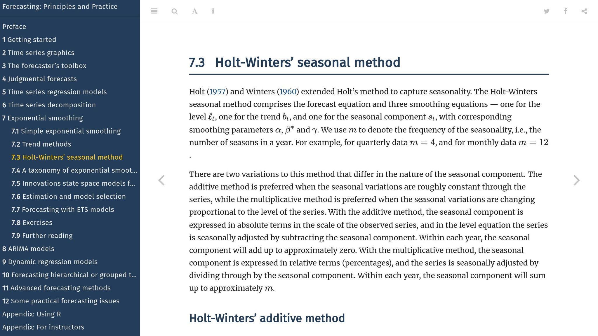
The Holt-Winters method, also known as triple exponential smoothing, builds on simpler forecasting techniques by accounting for trends and seasonal changes. It uses three smoothing equations to measure level, trend, and seasonality, making it a powerful tool for analyzing data with seasonal patterns.
There are two main variations of the Holt-Winters method:
- Multiplicative Method: Ideal for data where seasonal effects grow along with the trend. For example, in e-commerce, holiday sales often see larger seasonal spikes as overall sales increase over time.
- Additive Method: Best suited for data with consistent seasonal fluctuations, regardless of trend changes. A good example is electricity usage, where seasonal variations stay relatively stable even as overall usage trends shift.
The flexibility of this method makes it a strong choice for tackling complex forecasting scenarios.
Common Applications of Holt-Winters
- Energy usage forecasting: Analyzing seasonal cycles in consumption patterns.
- Tourism demand prediction: Estimating visitor numbers that rise seasonally while accounting for gradual growth.
- Retail forecasting: Capturing shifting seasonal patterns alongside long-term growth trends.
5. X-13ARIMA-SEATS
X-13ARIMA-SEATS combines ARIMA modeling with SEATS signal extraction to deliver more accurate demand forecasts through advanced seasonal adjustment techniques.
Core Components
The process starts with ARIMA pre-adjustment, which smooths out irregularities like calendar effects and holiday impacts. After that, SEATS decomposition breaks the data into three parts: trend-cycle, seasonal, and irregular components.
When to Use X-13ARIMA-SEATS
This method is best suited for analyzing long-term datasets that have intricate or multiple seasonal patterns, ensuring precise seasonal adjustments.
Implementation Considerations
To apply X-13ARIMA-SEATS effectively, you’ll need consistent historical data, statistical expertise, and adequate computing power. It works well as a supplement to earlier methods, offering a detailed breakdown of seasonal influences.
Method Selection Guide
To choose the best seasonal adjustment technique for your dataset, consider the nature of its seasonal patterns.
- Additive methods work well when seasonal effects remain steady over time.
- Multiplicative methods are better suited for cases where seasonal fluctuations grow or shrink in proportion to data levels.
- For datasets with more unpredictable trends, methods like moving averages, Holt-Winters, or X-13ARIMA-SEATS can handle the complexity effectively.
Use these guidelines as a quick reference while finalizing your forecasting approach.
Conclusion
We’ve explored various techniques, and the key takeaway is this: choosing the right seasonal adjustment method for your data is essential to identifying real trends and making informed decisions.
Using a data-focused approach can turn seasonal fluctuations into meaningful insights. As Growth-onomics puts it, "With Data as Our Compass We Solve Growth".
To ensure success, tailor your method to your business by considering:
- The complexity of your data and its historical trends
- Resources available for implementation
- The level of accuracy your forecasts require
- How well the method integrates with your analytics tools
Seasonal adjustment isn’t a one-time task. Regular reviews are necessary to keep your results precise and trustworthy.
"Our services revolve around a data-driven, results-focused methodology that leverages the most advanced technologies and best practices to help brands achieve their full potential." – Growth-onomics
These strategies provide a solid foundation for leveraging seasonal adjustment methods to support your business growth effectively.